The program is designed for tolerance analysis of linear (1D) dimensional chains. The program solves the following problems:
All solved tasks enable work with standardized tolerance values, both in designing and in optimization of the dimensional chain.
Data, methods, algorithms and information from professional literature and ANSI, ISO, DIN and other standards are used in calculation. List of standards: ANSI B4.1, ISO 286, ISO 2768, DIN 7186
![]()
User interface.
![]()
Download.
![]()
Purchase, Price list.
Information on the syntax and control of the calculation can be found in the document "Control, structure and syntax of calculations".
Information on the purpose, use and control of the paragraph "Information on the project" can be found in the document "Information on the project".
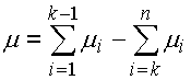
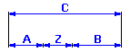
A linear dimensional chain is a set of independent parallel dimensions which continue each other to create a geometrically closed circuit. They can be dimensions specifying the mutual position of components on one part (Fig. A) or dimensions of several parts in an assembly unit (Fig. B).
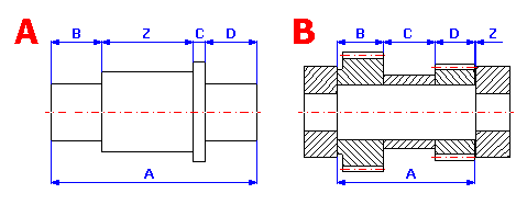
A dimensional chain consists of separate partial components
(input dimensions) and ends with a closed component (resulting
dimension). Partial components (A, B, C,…) are dimensions either directly
dimensioned in the drawing or following from previous manufacturing, possibly
assembly operations. The closed component (Z) in the given chain represents the
resulting manufacturing or assembly dimension, which is the result of combining
partial dimensions as a scaled manufacturing dimension, possibly assembly
clearance or interference of a component. The size, tolerance and limit
deviations of the resulting dimension depend directly on the size and tolerance
of partial dimensions. Depending on how the change of partial component affects
the change of the closed component, two types of components are distinguished in
dimensional chains:
- increasing components - partial components, the increase of
which results in an increase of the closed component
- decreasing components - partial components, the increase of
which results in a decrease of the closed component
When solving tolerance relations in dimensional chains, two types of problems occur:
The choice of method of calculation of tolerances and limit deviations of dimensional chain components affects manufacturing accuracy and assembly interchangeability of components. Therefore, economy of production and operation depends on it. To solve tolerance relations in dimensional chains, engineering practice uses three basic methods:
The most often used method, sometimes called the maximum - minimum calculation method. It works on the condition of keeping the required limit deviation of a closed component for any combination of real dimensions of partial components, i.e. also upper and lower limit sizes. This method guarantees full assembly and working interchangeability of components. However, due to the demand of higher accuracy of the closed component, it results in too limited tolerances of partial components and therefore high manufacturing costs. The WC method is therefore suitable for calculating dimensional circuits with a small number of components or in case that broader tolerance of the resulting dimension is acceptable. It is most often used in piece or small-lot production.
The WC method calculates the tolerance of the resulting dimension as an arithmetic sum of tolerances of all partial dimensions. The dimensions of a closed component are therefore determined by its mean value:
and total tolerance:

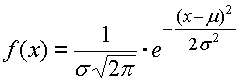
Boundary dimensions of the closed component are set by the relations:
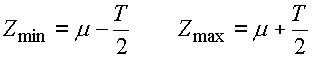
with:
mi - mean dimension of ith component
Ti - tolerance of ith component
n - total of partial components
i=1,..,k - number of increasing components
i=k,..,n - number of decreasing components
Statistical methods of calculation of dimensional chains are based on the calculus of probability. These methods assume that in a random selection of components during assembly, the limit values of deviations only rarely occur with more partial components simultaneously, as is the case of combined probability. The probability of the occurrence of limit value of deviations in manufacturing individual dimensions on one component will be similarly small. With a certain, pre-selected risk of rejection of some components, the tolerances of partial components in the dimensional chain can be increased.
The statistical method guarantees only partial assembly interchangeability, with a low percentage of unfavourable cases (spoilage). With respect to larger tolerances of partial dimensions, however, it results in a decrease in manufacturing costs. It is mainly used in mass and large-lot production, where savings in manufacturing costs outbalance increased assembly and operating costs resulting from incomplete assembly interchangeability of components.
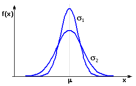
The dimensions of a closed component show certain variation from the mean of the tolerance field. The frequency of occurrence of individual dimensions follows the rules of mathematical statistics and in the outright majority of cases it matches normal distribution. This distribution is described by the Gauss curve of probability density, for which the frequency of occurrence of "x" dimension follows the relation:
The shape of the Gauss curve is characterized by two parameters. Mean value m determines the position of maximum frequency of the resulting dimension occurrence; standard deviation s defines the curve "slenderness".
The area defined by the intersection of the Gauss curve with the required closed component limit dimensions represents the expected yield of the process. Parts of the curve lying outside the tolerance interval define the area which represents spoilage in the process.
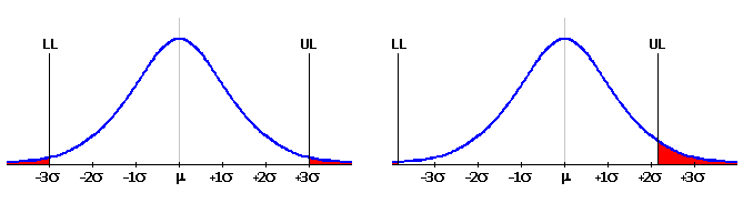
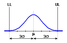
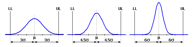
In general engineering, the manufacturing process is usually considered satisfactorily efficient on the level 3s. That means that the upper limit UL and lower limit LL of the resulting dimension is at 3s distance from the mean value m. The area of the Gauss curve between both limits then equals 99.73% of the total area and represents the portion of products meeting the specification requirements. The area outside these limits equals 0.27% and represents off-size products.
| Limit sizes | Process yield [%] | Number of rejects per million components produced |
| m ± 1s | 68.2 | 317310 |
| m ± 2s | 95.4 | 45500 |
| m ± 3s | 99.73 | 2700 |
| m ± 3.5s | 99.95 | 465 |
| m ± 4s | 99.994 | 63 |
| m ± 4.5s | 99.9993 | 6.8 |
| m ± 5s | 99.99994 | 0.6 |
| m ± 6s | 99.9999998 | 0.002 |
This method of calculation is a traditional as well as the most widespread method of statistical calculation of dimensional chains. The RSS method is based on the assumption that individual partial components are manufactured with the level of process capability (quality) 3s.
Their limit values therefore match tolerance interval m ± 3s, and standard deviation is set by the relation:

The dimensions of a closed component are determined by its mean value:
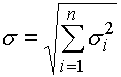
and standard deviation:
with:
si - standard deviation of ith
component
mi - mean dimension of ith component
Ti - tolerance of ith component
n - total of partial components
i=1,..,k - number of increasing components
i=k,..,n - number of decreasing components
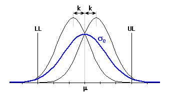
In general engineering, the manufacturing process was traditionally considered satisfactorily efficient on level 3s. That means an estimated 2700 rejected products per one million produced. Although such portion of off-size products seems very good at first sight, it is considered ever more and more insufficient in some spheres of production. Besides, it is almost impossible to keep the mean value of the process characteristic curve exactly in the middle of the tolerance field in the long term. In case of large production volumes, the mean value of the process characteristic shifts in the course of time due to the influence of various factors (erroneous set-up, wear of tools and jigs, temperature changes, etc.). A shift of 1.5s from the ideal value is typical. In case of traditionally approached processes with 3s level of capability, that represents an increase of the off-size product ratio to approx. 67000 per one million produced.
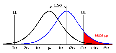
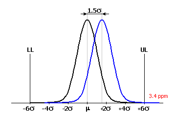
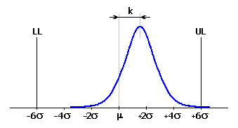
It is obvious that a manufacturing process with such level of spoilage is unacceptable. Therefore, recently the modern "6 Sigma" method has been used more and more frequently to assess the quality of manufacturing processes. The concept of the method is to achieve such target that the mean value of the process characteristic is at 6s distance from both tolerance limits. In such efficient manufacturing process, the ratio of 3.4 off-size products per one million produced is achieved even after the expected mean shift of 1.5s.
The "6 Sigma" method is relatively new; it became popular rather broadly only in the 1980s and 1990s. It was put into practice for the first time by Motorola and it is considerably used mainly in the USA. Its utilization is suitable in case a higher quality of manufacturing processes is required and for large production volumes where the mean value of the process characteristic may be shifted.
The "6 Sigma" method is a modification of the standard "RSS" method and introduces two new parameters, (Cp, Cpk), called process capability indexes into the problems of dimensional chain solutions. These capability indexes are used to assess the manufacturing process quality.
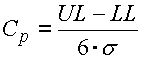
The Cp capability index assesses the quality of the manufacturing process using the comparison of specified tolerance limits with the traditional capability level 3s.
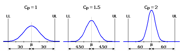
For the process with tolerance interval m ± 3s, Cp will equal 1. With high quality processes where tolerance limits are at ±6s distance from the mean value, the capability index will be Cp=2.
The Cpk index is a modified Cp index for mean shift of the process characteristic.
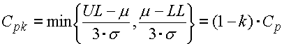
where the mean shift factor k ranges between <0..1> and determines the relative value of the mean shift related to half of the tolerance interval. In case of a typical mean shift of process characteristic of 1.5s, the mean shift factor for the process with "6 Sigma" quality will be k=0.25 and the capability index Cpk=1.5.
The effective standard deviation of the process may then be estimated as:
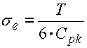
After the application of capability indexes on all partial components of the dimensional chain, the dimensions of the closed component can be described similarly to the "RSS" method by its mean value m and standard deviation:
with:
sei - effective standard deviation of ith component
In case of the "6 Sigma" method, a manufacturing process with resulting 4.5s capability ratio is typically considered satisfactory.
The selective assembly method is used in mass and large-lot production of precise products which do not require working interchangeability of components inside the product. The assembly of the product is preceded by sorting of individual components into tolerance subsets. Manufacturing dimensions of components may be prescribed with a larger tolerance. The narrowed resulting dimensional tolerance is achieved by the functional matching (combination) of sorted subsets. To determine the resulting dimension of the closed component, the above-specified "WC" method is used, except that the calculation does not include all manufacturing tolerances of partial components, but only narrowed tolerances applicable for the selected tolerance subset.
The selective assembly method is a very effective method of solving dimensional chains, enabling a substantial increase in manufacturing tolerances of partial components and thus a significant reduction in manufacturing costs. On the other hand, application of this method places increased demands on product assembly. Operating costs will also increase, as it is usually necessary to replace the whole assembled component in case of wear or damage of a partial component.
If the selective assembly method is to be effective, it is necessary to solve the problem of optimum selection (combination) of components. The components have to be matched so that it is possible to assemble the maximum possible number of products meeting the functional requirements with the given number of manufactured components. This task can be divided into two parts:
Finding all combinations of individual subsets of partial components for which the functional requirements are met by the closed component.
This task has to be solved before the beginning of production, in the process of designing the dimensional chain. The number of suitable combinations will depend on the overall manufacturing tolerance of partial components, as well as the selected number of tolerance subintervals. The dimensional chain should be designed so that the number of acceptable assembly combinations ranges within reasonable limits.
For small numbers of suitable combinations, it will probably not be possible to use all manufactured parts during the assembly. That is why the assembly yield of the process decreases and the production becomes more expensive. The critical index is represented by the state when some of the subsets appear unacceptable already in the design stage.
On the other hand, a large number of suitable combinations signal an ineffective design. The tolerance chain could probably be designed in a more optimal way, with larger tolerances of partial components or with a smaller number of tolerance subintervals.
Optimization of the number of assembled products for the given numbers of manufactured components in individual tolerance subintervals.
This task has to be solved repeatedly during production, always before replenishing the stock before the beginning of assembly itself. The main aim of the task is to determine the optimum assembly procedure in order to achieve the biggest possible number of assembled products. When solving the task, we have to choose the optimum set of combinations from the subset of acceptable combinations used in assembly and at the same time determine the number of products assembled within each used combination.
The algorithm of optimization is based on gradual assembly of individual products by retracting the components from selected subsets. In the first stage, the calculation estimates the minimum and maximum possible number of assembled products. In further stages it retracts the parts from the selected subsets according to a pre-selected scheme so that the lower estimate of the number of assembled products increases as fast as possible and the upper estimate decreases as slowly as possible.
The solution to the task usually is not unambiguous. Several different assembly procedures leading to an identical number of assembled products can often be found. That is why the number of used assembly combinations is used as another optimization criterion. The minimization of the number of used combinations results in simplification and speeding-up of assembly, i.e. in the reduction of manufacturing costs. In some practical applications, both criteria are identically important.
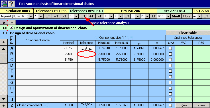
This line is used to switch over the system of units for calculation and to select standardized tolerances.
In the list box, select the required system of units for calculation. After switching the units, all values will be automatically recalculated.
When defining the dimensional chain in paragraphs [1.1, 3.2, 5.1, 7.1], the tolerance is also set for each dimension. To simplify work, the program is provided with a tool for automatic selection of standardized tolerances.
The program includes a set of basic dimensional tolerances according to ISO, or ANSI. With respect to the type of deviation and applied standard, the tolerances are divided into 5 subsets:
Each subset contains a set of list boxes and buttons in the heading of the workbook. Set the required parameters of tolerance, possibly fits (accuracy level, tolerance field, ..) in the list boxes. Using the buttons, insert the dimensions of the required deviation into the appropriate place in the input table - the line with the active cell.
Tolerances according to ISO are defined by the standard in [mm] and are intended for calculation in SI units. Tolerances according to ANSI are defined in [in] and are intended for calculation in Imperial units. In case of use of standardized tolerances defined in units other than those set in the calculation, the deviations of the dimension will be automatically recalculated and rounded.
This chapter enables the tolerance analysis, synthesis and optimization of dimensional chain using the arithmetic "WC" method, possibly statistic "RSS" method to be performed.
The "Worst Case" method is used in case full assembly and working interchangeability of components is required and is suitable for solving dimensional circuits with a small number of components or if rougher tolerance of the final dimension is acceptable. The statistical "Root Sum Squares" method guarantees only partial assembly interchangeability and is used to decrease manufacturing costs in mass and large-lot production.
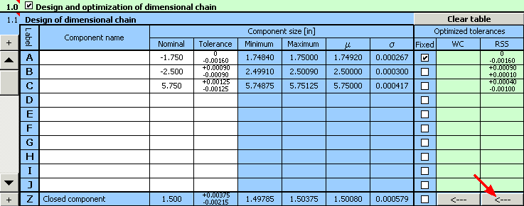
The task of designing and optimization of a dimensional chain consists of the following steps:
This paragraph is intended for the design of a dimensional chain and optimization of tolerances of selected partial components.
This table is used to define the dimensions of individual partial components of a dimensional chain. Each line of the table belongs to one partial component. The meaning of the table is obvious from the following description:
Column 1 - Name of component is an optional parameter.
Column 2 - Set the nominal dimension of partial component.
"Increasing" components are positive, "decreasing"
components are set with negative value.
Column 3 - Set upper and lower deviation of the dimension. Press the
selected button in the heading of the workbook to insert the deviations
appropriate to the selected tolerance into the table.
Column 4..7 - These columns contain the calculation of limit sizes, mean
dimension and standard deviation of all partial components.
Column 8 - Set the switches to mark all partial components with
tolerances to be optimized. Checking the field marks fixed tolerance, which will
remain without changes after optimization.
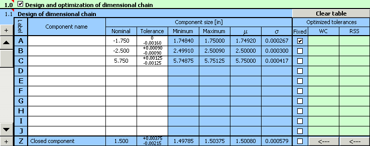
Column 9,10 - After optimization, these columns contain designed
(optimized) deviations. The left column contains results of optimization using
the arithmetic "WC" method; the right one contains the results using
the statistical "RSS" method. Press the button located on the bottom
line of the table to transfer the designed deviations into the input column.
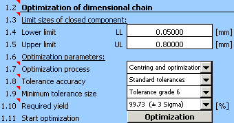
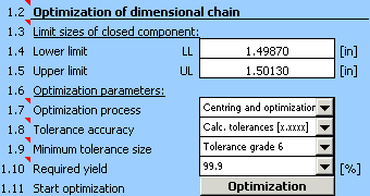
This paragraph is used to optimize tolerances of selected partial components of the dimensional chain defined in table [1.1]. Before the beginning of optimization, set the required limit sizes of the closed component [1.3] and set optimization parameters [1.6]. Start optimization using the button in line [1.11].
Optimization is performed for both calculation methods (WC, RSS) simultaneously. Designed deviations are listed in table [1.1], for resulting dimensions of the closed component see paragraph [2].
This paragraph defines required limit sizes of the closed component determined by functional requirements of the product.
Select one of the following optimization modes in the list box:
1. Design centring
With the size of tolerance preserved, the calculation will adjust limit
deviations of selected partial components so that the mean dimension of the
closed component is as close to the mean of the required tolerance interval
determined by limits [1.3] as possible. Depending on the set-up of tolerance
accuracy [1.8], the calculation works in two modes:
2. Optimization of tolerances
With the mean value of the tolerance interval preserved, the calculation adjusts
the tolerance of selected partial components so that the resulting dimensions of
the closed component meet the requirements of the specification determined by
limits [1.3].
3. Centring and optimization
Combination of both previous procedures
In the list box select the type and accuracy of tolerances used during optimization.
In case any of first five items in the list box are selected, the size of the optimized tolerance will be set by the calculation, with a predetermined level of accuracy (number of decimal places). For optimized tolerances, the mutual ratio of their sizes is kept.
In case the remaining two items in the list box are selected, the size of optimized tolerances will match standardized values. For calculation in SI units, standardized tolerances according to ISO 286 are used, for calculation in Imperial units they are used according to ANSI B4.1. In case the "Same tolerance grade" item is selected, the standardized tolerances from the same tolerance grade will be used for all optimized dimensions.
Set the minimum size (accuracy grade) of tolerances which can be used during optimization.
Choose the minimum required yield of the manufacturing process from the list box.
This paragraph presents in a well-arranged form the detailed parameters of a closed component for the dimensional chain defined in paragraph [1]. For comparison, it contains the resulting dimensions of closed components for both original and optimized tolerances of partial components.
In this paragraph, define the required limit sizes of the closed component given by functional requirements of the product.
This paragraph shows resulting dimensions of the closed component in case the arithmetic "Worst Case" calculation method is used.
This paragraph shows parameters of the closed component in case the statistic "Root Sum Squares" calculation method is used.
Productive yield [2.13] specifies the expected ratio of products meeting the specification requirements, i.e. products with a resulting closed component dimension within the interval specified by limit sizes [2.1]. Rejection of the manufacturing process [2.14] represents the estimated number of off-size products per million produced products.
This paragraph contains the calculation of limit sizes of the closed component for the selected yield of the manufacturing process.
The calculation used in chapter [A] is based on the assumption that the designed component will work at temperatures close to the basic temperature of 20°C (68°F) that the dimensions and tolerances of partial components were set at. If the components operate permanently at higher working temperatures, their dimensions are deformed during operation. This chapter is therefore meant to analyse the linear dimensional chain deformed as a result of the working temperature change. To check the resulting dimension of the closed component, the arithmetic "WC" or statistic "RSS" methods can be used.
In this paragraph, define the dimensional chain and working temperature for the operation of the designed component.
Set the expected working temperature for the operation of the designed component.
This table is used to define the dimensions of individual partial components of the dimensional chain. One line of the table belongs to each partial component. The meaning of columns in the table is obvious from the following description:
Column 1 - Name of component is an optional parameter.
Column 2 - Set the nominal dimension of the partial component.
"Increasing" components are positive; set the "decreasing"
components with negative value.
Column 3 - Set the upper and lower deviation of the dimension. Press the
selected button in the workbook heading to insert the deviations appropriate to
the selected tolerance into the table.
Column 4,5 - Manufacturing (assembly) dimensions of partial components
are calculated in these columns.
Column 6 - Select the material of the component in the list box.
Column 7 - Set the heat expansion coefficient. If the check box in the
table heading is checked, the values will be set automatically according to the
selected material and working temperature [3.1].
Column 8,9 - In these columns, dimensions of partial components at
working temperature are calculated.
This paragraph shows in a well-arranged form the detailed parameters of a closed component for the dimensional chain defined in paragraph [3]. For comparison, the resulting dimensions of the closed component during assembly (20° C) and at working temperature are given here.
Set the coefficient of heat expansion of the closed component material.
In this paragraph define the required assembly dimensions of the closed component. Limit sizes of the closed component at working temperature are calculated automatically in dependence on the selected heat expansion coefficient [4.1].
This paragraph shows resulting dimensions of the closed component in case the arithmetic "Worst Case" calculation method is used.
This paragraph shows parameters of the closed component in case the statistic "Root Sum Squares" calculation method is used.
Productive yield [4.15] specifies the expected ratio of products meeting the specification requirements, i.e. products with a resulting closed component dimension within the interval specified by limit sizes [4.3]. Rejection of the manufacturing process [4.16] represents the estimated number of off-size products per million produced products.
This paragraph contains the calculation of limit sizes of the closed component for the selected yield of the manufacturing process.
This chapter enables tolerance analysis of a linear dimensional chain using the statistical "6 Sigma" method to be performed.
The "6 Sigma" method is a modern statistical method used for the assessment of manufacturing process quality. It is especially suitable in case of a requirement for higher quality manufacturing processes and for large volumes of production, where the mean value of the process characteristic may be shifted. The objective of the method is to achieve the mean value of the process characteristic at 6s distance from both tolerance limits. For such capable manufacturing process, the rate of 3.4 off-size products per million manufactured is achieved even at the expected mean shift.
This paragraph is meant for the design of a dimensional chain.
This table is used to define the parameters of individual partial components in a dimensional chain. One line of the table belongs to each partial component. The meaning of columns in the table is obvious from the following description:
Column 1 - Name of component is an optional parameter.
Column 2 - Set nominal dimension of partial component.
"Increasing" components are positive; set the "decreasing"
components as a negative value.
Column 3 - Set upper and lower deviation of the dimension. Press the
selected button in the heading of the workbook to insert the deviations
appropriate to the selected tolerance into the table.
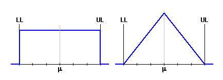
Column 4 - In the list box choose the type of theoretical frequency
distribution. As a standard, normal distribution, which best
matches the real distribution of random process quantities in the outright
majority of cases, is used to describe the manufacturing processes.
Column 5 - Set the capability index of the manufacturing process. If
the check box in the table heading is checked, the values appropriate to the
selected type of theoretical frequency distribution will be used automatically.
Column 6 - Set the factor of the process characteristic mean shift. This
factor determines the relative value of mean shift related to half the tolerance
interval. For a manufacturing process with "6 Sigma" quality, the mean
shift factor k=0.25 is usually used.
Column 7 - In this column, the modified index of capability is calculated
for the mean shift of the process characteristic.
Column 8,9 - In these columns, the mean value and effective standard
deviation of the process are calculated.
In this paragraph, the detailed parameters of the selected input component are presented numerically and graphically in the way it was defined in table [1.1].
This paragraph shows in a well-arranged form the detailed parameters of a closed component for the dimensional chain defined in paragraph [5].
In this paragraph, define the required limit sizes of the closed component given by functional requirements of the product.
This paragraph shows the parameters of a closed component using the statistical "6 Sigma" calculation method.
Productive yield [6.11] specifies the expected ratio of products meeting the specification requirements, i.e. products with a resulting closed component dimension within the interval specified by limit sizes [6.1]. Rejection of the manufacturing process [6.12] represents the estimated number of off-size products per million produced products.
This paragraph contains the calculation of limit sizes of the closed component for the selected yield of the manufacturing process.
This chapter enables tolerance analysis of a linear dimensional chain using the group interchangeability (selective assembly) method to be performed.
The selective assembly method is used in mass and large-lot production of precise products which do not require working interchangeability of components within the product. Product assembly is preceded by the sorting of individual components into tolerance subsets. Manufacturing dimensions of components can be prescribed with bigger tolerance. Narrowed tolerance of the resulting dimension is achieved by practical matching (combination) of sorted subsets.
The task of designing the dimensional chain consists of the following steps:
Besides the dimensional chain design itself, the optimization of a number of assembled products for the specified numbers of manufactured components [9] is usually a part of the solution. This task has to be solved repeatedly during production, whenever the stock is replenished before the beginning of assembly.
This paragraph is intended for designing and check of dimensional chain.
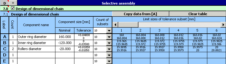
In table [7.1] define the number, dimensions and tolerances of all components that the final product will be assembled from. Further select the number of tolerance subsets (subintervals) for each component that the component will be sorted into before the assembly. In paragraph [7.2] you will find the limit sizes of the closed component for any assembly combination of sorted component subsets.
This table is used to define the dimensions of individual partial components (parts) of the dimensional chain. One line of the table belongs to each component. The meaning of columns in the table is obvious from the following description:
Column 1 - Set the number of identical components joining the
dimensional chain.
Column 2 - Name of component is an optional parameter.
Column 3 - Set the nominal dimension of the partial component.
"Increasing" components are positive; set the "decreasing"
components as a negative value.
Column 4 - Set the upper and lower dimensional deviation. Press the
selected button in the workbook heading to insert deviations appropriate to the
selected tolerance into the table.
Column 5 - Set the number of tolerance subsets (subintervals) that the
component will be sorted into. You will set the identical number of subsets for
all components using the selection from the list box in the table heading.
Column 6..11 - In these columns the limit sizes of all tolerance
subintervals are calculated. Individual subsets are marked with a numerical
index in the heading of table. Together with the component marking, the index is
used to unambiguously describe the selected assembly subset (A1, A2, B1, B2, B3,
...).
In the first line of the table, the limit dimensions of the closed component determined by the "Worst Case" method for full tolerances of partial components are specified. This data is only informative and is significant mainly for design centring. In case of well and efficiently performed design of a tolerance chain, the mean dimension specified here should be as close to the required dimension [8.7] as possible.
In the second line you will find the limit sizes of the closed component for any assembly combination of sorted component subsets. You can set the required assembly combination using the appropriate tolerance subsets in list boxes.
Solving the task of correct component pairing is an inseparable part of designing a dimensional chain. The purpose of this task is to find such assembly combinations of individual component subsets for which the closed component meets the functional product requirements. The total of found combinations is the criterion for assessment of the design quality. The dimensional chain should be designed so that the number of suitable assembly combinations ranges within reasonable limits.
For small numbers of suitable combinations, it will probably not be possible to use all manufactured parts during assembly. That way the assembly yield of the process decreases and production becomes more expensive. The critical index is the state when some subsets seem unacceptable already in the design stage.
On the other hand, a large number of suitable combinations signal an ineffective design. The tolerance chain could probably be designed in a more optimal way, with larger tolerances of partial components or with a smaller number of tolerance subintervals.
The selective assembly method guarantees only partial (group) assembly interchangeability within the selected assembly combinations. In case of wear or damage of a partial component during operation, it is necessary to replace the whole assembled component. That is why the selective assembly method is used especially in the production of precise products, when working interchangeability of components inside the product is not required.
Although it will result in increased manufacturing costs, it may still be more economically advantageous in case of some products to ensure complete working interchangeability of at least one component. For such defined requirement, we can apply two different solutions (methods) when solving the task of selective assembly:
In this paragraph, define the required limit sizes of the closed component determined by the functional requirements of the product. The first column shows limit sizes of the closed component during product assembly. The second column shows limit sizes when the selected component is replaced.
This paragraph is used to search for all assembly combinations for which the closed component meets the functional requirements of the product specified in paragraphs [8.1, 8.4]. The program works in two modes:
Set the search mode in list box [8.9]. Run the search using the button in line [8.10], results are specified in paragraph [8.11].
This parameter specifies the total of all assembly combinations that can be used in assembly of the product.
This parameter specifies the number of all found assembly combinations for which the closed component meets the functional requirements of the product specified in paragraphs [8.1, 8.4]. The total of found combinations is then the criterion for the design quality assessment. The dimensional chain should be designed so that the number of suitable assembly combinations ranges within reasonable limits.
For small numbers of suitable combinations, it will probably not be possible to use all manufactured parts during assembly. That way the assembly yield of the process decreases and production becomes more expensive.
On the other hand, a large number of suitable combinations signal an ineffective design. The tolerance chain could probably be designed in a more optimum way, with larger tolerances of partial components or with a smaller number of tolerance subintervals.
The table of suitable combinations shows assembly combinations with the closed component meeting the functional requirements of the product specified in paragraphs [8.1, 8.4]. The resulting dimensions of close component for the selected combination are specified in paragraph [8.15].
The table of unused subsets shows all tolerance subsets (subintervals) for which no acceptable assembly combination can be found. Products sorted into these subsets cannot be used during assembly. The assembly yield of the process decreases and production becomes more expensive. For a correctly designed dimensional chain, this table should remain empty.
This paragraph numerically and graphically presents the resulting dimensions of the closed component for the assembly combination selected in table [8.14]. The first column shows limit sizes of the closed component during assembly. The second column gives the limit sizes in case the selected component is replaced.
If the selective assembly method is to be effective, it is necessary to solve the problem of optimal choice (combination) of components. The components have to be matched so that it is possible to assemble the maximum possible number of products meeting the functional requirements using the given number of manufactured components.
This task has to be solved repeatedly during production, whenever the stock is replenished before assembly itself is started. The main part of the task is to determine an optimum assembly procedure in order to achieve the largest possible number of assembled products. When solving the task, we have to choose the optimum set of combinations from the subset of acceptable combinations [8.14] used in assembly and at the same time determine the number of products assembled within each used combination.
The solution to the task is not usually unambiguous. It is often possible to find several different assembly procedures leading to an identical number of assembled products. That is why the number of used assembly combinations is used as another optimization criterion. The minimization of the number of used combinations results in simplification and speeding-up of assembly, i.e. a reduction in manufacturing costs. In some practical applications both criteria are identically important.
Set numbers of manufactured components in individual tolerance subintervals in the table.
Select the required optimization method from the list box.
Besides the demand to assemble the maximum number of products, the demand to minimize the number of assembly combinations which will be used for assembly of the product often occurs in practice. With a decreasing number of used combinations, however, the total of assembled products also decreases. It is obvious that both these demands are antagonistic. Therefore, the parameter specifying the weight (importance) of individual criteria has to be specified during optimization. Set the mutual rate of importance of both criteria using the scroll bar.
The solution of the problem of optimization of the number of assembled products is not usually unambiguous. Several different assembly procedures resulting in the same number of assembled products can often be found. Therefore, the calculation offers the choice of selecting from several different solutions put together using different optimization schemes (algorithms). Select the solution in the list box before running the optimization.
In this paragraph you can find the basic qualitative parameters of the designed assembly procedure. A detailed specification of the optimized assembly procedure can be found in table [9.12].
This table shows the detailed specification of an optimized assembly procedure. The left column shows all assembly combinations used for the product assembly. The right column gives the number of products assembled within each combination.
This table shows the numbers of remaining (unused) components which could not be used in product assembly.
For the illustration of problems of tolerance analysis of linear dimensional chains, the user's guide is provided with several practical examples of utilization of this calculation:
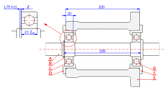
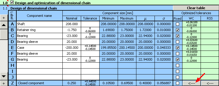
For the example of fit of the shaft in the case (see the picture), design manufacturing tolerances of individual components so that 0.05 - 0.80 mm clearance in fit is ensured. The designed tolerances have to match the following technological production requirements:
- contact areas of the case will be machined using milling
- turning will be used to machine the shaft and bearing bushings
with:
A ....... Shaft
B ....... Retainer ring 40 DIN 471
C,G .... Bearing 6308 DIN 625 SKF
D,F .... Bearing sleeve
E ....... Case
Z ....... Clearance in fit <0.05 to 0.80> mm
If we start from the dimensional chain diagram
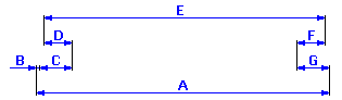
we can describe clearance in fit for the given problem using the relation Z = A - B - C + D - E + F - G
In the design of manufacturing tolerances itself we have to proceed from the technological demands of production. The size of designed tolerances of individual components has to range within the manufacturing accuracy achievable with the selected machining method. In case of milling, commonly achieved manufacturing accuracy ranges between tolerance levels 9 and 13, in case of turning it ranges between tolerance levels 6 and 12.
We can divide the solution of the task of designing and optimization of a dimensional chain into the following steps:
1) Using the above-mentioned relation, we will define the dimensional chain in table [1.1]. Partial components of the chain are formed by individual components; required clearance in fit is the closed component of the dimensional chain.
2) In case of components with fixed tolerance prescribed by the manufacturer (bearings, retained ring), we will set the appropriate dimensional deviations in the input table.

3) Contact areas of the case will be machined by milling; in the first design we will therefore select the size of tolerance at accuracy level 11 for the width of the case.
4) By checking appropriate switches in column 8 of the table, we will mark all components with fixed tolerance.
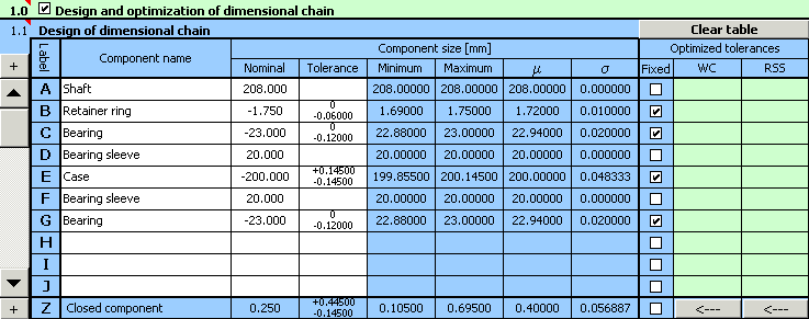
5) In paragraph [1.3] we will set limit values of the required clearance in fit.
6) In list box [1.7] select the "Centring and optimization" method, in list [1.8] choose "Standard tolerances".
7) Turning will be used to machine all components for which we want to design tolerances in the next step. In the list box [1.9] we will therefore set the minimum allowed number of tolerance to accuracy level 6.
8) Using the button in line [1.11] we will start optimization of the dimensional chain.
9) Parameters of the resulting clearance achieved for the optimized design of tolerances are shown in paragraph [2.5],
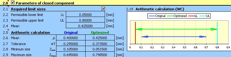
optimized deviations of manufacturing dimensions are listed in column 9 of table [1.1].
10) For the example specified herein, a functionally suitable solution was found during optimization; however from the practical point of view such design is not suitable. The program designed the width of the bearing sleeves in lines D and F with different tolerances. For the sake of production and assembly efficiency, it is necessary to secure interchangeability of both bearing sleeves. The next step in the design deals with removing this fault.
11) Use the button on the bottom table line to transfer the designed tolerances to the input part of the table, then unify the tolerance for both sleeves using the higher of the designed values.

12) In column 8 of the table, further check the switches in lines D and F, and restart optimization using the button on line [1.11].
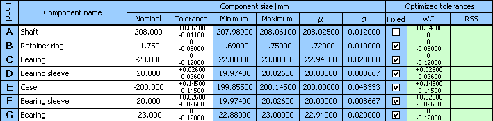
13) This time the design will result in a fully suitable solution of the problem with bearing sleeve tolerance at accuracy level 9 and accuracy level 7 for shaft tolerance.
The solution designed herein will not of course be the only suitable solution to the problem and it need not be the ideal solution either. Therefore, it is appropriate (especially in case of lot production) to design several different solutions with varying accuracy of manufacturing of individual components.
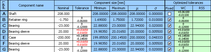
We will obtain another solution to the problem if we choose the lower of the originally designed values for the bearing sleeve tolerance in step 11).
We will obtain further suitable solutions in case of selecting a different case width in step 3). The following table shows a comparison of several suitable designs:
| Solution 1 | Solution 2 | Solution 3 | Solution 4 | |
| Tolerance grade | ||||
| Case | 11 | 11 | 10 | 10 |
| Bearing sleeves | 9 | 8 | 10 | 9 |
| Shaft | 7 | 8 | 8 | 9 |
| Clearance in fit [mm] | 0.053 - 0.793 | 0.061 - 0.789 | 0.062 - 0.788 | 0.073 - 0.777 |
The resulting solution has to be chosen so that the total manufacturing costs are as low as possible.
For the component (see picture), design the manufacturing tolerances of dimensions so that the permissible deviation ±0.0013 in for the technologically resulting dimension is not exceeded.
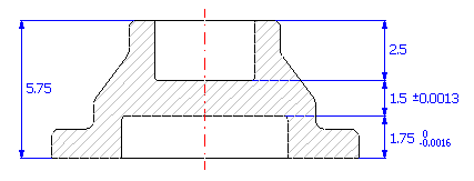
If we start from the diagram of the dimensional chain
we can describe the resulting dimension for the given component using the relation Z = C - A - B.
If the problem were solved using the common "Worst Case" method, it would be necessary to use tolerance at approx. accuracy level 4 for dimensions B and C to keep the required tolerance of the resulting dimension. It is obvious that production with such accuracy level would be unreasonably expensive. In this case it will therefore be much more advantageous to use the statistical method of calculation. This method enables manufacturing of a component with significantly greater tolerances, at the cost of a low (pre-selected) percentage of spoilage.
The solution to the task of dimensional chain design and optimization can be divided into the following steps:
1) Using the above-mentioned relation, we will define the dimensional chain in table [1.1].
2) We will further set the required manufacturing tolerances for individual dimensions. We will set the appropriate deviations for dimension A required by the task.
For the remaining dimensions we will tentatively select symmetrical tolerance at accuracy level 8.
3) In column 8 of the table, check the switch with dimension A, the tolerance of which is strictly given.
4) In paragraph [1.3] set the required limit values of the resulting dimension.
5) In list box [1.7] choose the "Centring and optimization" method, in list [1.8] set the required accuracy (number of decimal places) designed by the tolerance.
6) With respect to the various methods of machining applicable during production of the component, set the minimum allowed tolerance to accuracy level 6 in the list box [1.9].
7) In list box [1.10] choose the required production yield 99.9%, i.e. manufacturing process with maximum number of 1000 rejects per million manufactured components.
8) Start optimization of the dimensional chain using the button in line [1.11].
9) The resulting design parameters are shown in paragraph [2.10],

optimized deviations of manufacturing processes are shown in column 10 of table [1.1].
10) The designed tolerances can of course be further adjusted. Using the button on the bottom line of the table, transfer the optimized values of tolerances into the input part of the table. There, while keeping the tolerance sizes, we can e.g. finely tune the designed deviations to a more suitable shape.
Calculation results for this adjustment will be the same as the result achieved for the optimized tolerances.
The solution designed here will not of course be the only suitable solution to the problem and need not therefore be the ideal solution. When choosing a suitable solution, it is necessary to assess the relationship between the chosen sizes of manufacturing tolerances and expected manufacturing process yield. By increasing the applied tolerances we will achieve a decrease in direct costs connected with machining of the components, but it will result in an increase in losses due to the increased occurrence of faulty products. It is necessary to choose the resulting solution so that the total manufacturing costs are as low as possible.
For comparison, the following table shows the values of expected production yield for normalized tolerances of dimensions B and C.
|
Tolerance grade |
Expected production yield [%] |
Number of rejects per million manufactured components |
|
6 |
99.99 |
125 |
|
7 |
99.77 |
2324 |
|
8 |
97.54 |
24640 |
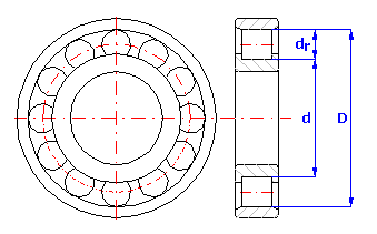
For a roller bearing assembled from three components with dimensions:
1. Outer ring - diameter D=160 mm
2. Inner ring - diameter d=120 mm
3. Rollers - diameter dr=20 mm
design the manufacturing tolerances of all components and parameters of the selective assembly so that a radial clearance ranging from 60 mm to 90 mm is kept during the bearing assembly. The bearing further requires interchangeability of the inner ring so that a radial clearance ranging from 40 mm to 105 mm is guaranteed during replacement of the ring in case of repair of the bearing.
Production of roller bearings is a typical example suitable for use of the selective assembly method. Using the traditional "Worst Case" method for the solution of the specified example will secure full assembly and working interchangeability of all components, however it would be necessary to manufacture the components of the bearing with accuracy level 3 to keep the required radial clearance. It is obvious that production with such accuracy level would be unreasonably expensive. Using the selective assembly method, the components can be made with significantly lower accuracy. The solution to the selective assembly problem itself consists of two parts:
The size of radial clearance for roller bearings is specified by the relation c = D - d - 2*dr.
The solution to the task of dimensional chain design and optimization can be divided into the following steps:
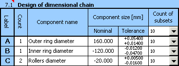
1) Using the above-mentioned relation, we will define the dimensional chain in table [7.1]. Individual components used during assembly of the bearing are partial components of the chain. The required radial clearance is then the closed component of the dimensional chain.
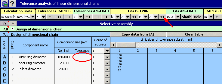
2) Next set the required manufacturing tolerances for individual dimensions. In the initial design, use tolerances at accuracy level 7 for all components. For the roller diameter, choose symmetric tolerance, H7 for the outer ring diameter tolerances and h7 for the inner ring.
3) For all components, initially set 10 tolerance subsets for the manufactured components to be sorted into.
4) In paragraph [8.1] set the requirement of working interchangeability of the inner bearing ring.
5) In paragraph [8.4] set limit sizes of the required radial clearance during assembly of the bearing and replacement of the inner ring.
6) In list box [8.9] choose search for all assembly combinations. Start the search for combinations using the button on line [8.10].
7) The design quality can be assessed from the results in paragraph [8.11]. It is obvious that in this case the design is not suitable. From the table of "Unused subsets" in line [8.14] it is clear that it was not possible to use more than half of the manufactured outer rings and rollers for assembly of the bearing.
8) For the unsuitable design, the next logical step could be decreasing the sizes of used manufacturing tolerances. On closer scrutiny of the design, however, we will find out that the main problem is not the selected size of tolerances, but rather wrong centring of the design. The standard indicator for better assessment of this design aspect is the mean dimension of the closed component calculated in paragraph [7.2].
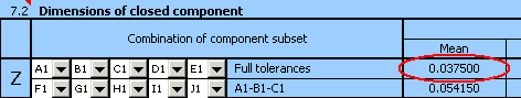
For the optimum design of the tolerance chain, the specified dimension should be as close to the required value as possible [8.7].
9) In the repeated design, adjust the position of the tolerance field of all components while keeping the sizes of tolerances. For the outer ring diameter, use G7 tolerance, and g7 for the inner ring diameter.
Next adjust the upper and lower deviation of the diameter of the rollers so that the resulting design is centred as well as possible.
10) For such adjusted design of a dimensional chain repeat the search for all suitable assembly combinations.
11) From the search results it is obvious that all manufactured components will be usable in the bearing assembly. However, the design is not that efficient as the number of suitable assembly combinations is unnecessarily high. We can decrease the number of suitable combinations e.g. by decreasing the number of tolerance subsets which the manufactured components will be sorted into.
12) While gradually decreasing the number of subsets, we will come to the resulting design of the dimensional chain,
which seems optimum for the selected example.
The resulting 75 suitable assembly combinations are acceptable for the purpose of selective assembly.
In the previous part of the task we designed manufacturing tolerances of components and searched for all suitable assembly combinations which can be applied during assembly of the bearing with suitable parameters. However, during the assembly itself it is not practical to assemble the bearings by mere random choice of components within permissible assembly combinations. If the selective assembly method is to be efficient, it is necessary to solve the problem of optimum selection (combination) of components. The components have to be matched so that it is possible to assemble the maximum possible number of products which meet the functional requirements with the given number of manufactured components.
This task has to be solved repeatedly during production, whenever the stock is replenished before assembly itself is started. The main part of the task is to determine the optimum assembly procedure in order to achieve the largest possible number of assembled products. When solving the task, we have to choose the optimum set of combinations from the previously found subset of acceptable combinations used in assembly and at the same time determine the number of products assembled within each used combination.
The solution to the task of optimization of the number of assembled products is performed in the following steps:
1) In table [9.1] set the number of manufactured components in individual tolerance subsets.

2) In list box [9.3] choose a suitable optimization method. For the selected example choose "Basic method", which gives the best results. Although this method is rather slower than the other methods for the small numbers of components which the bearing should be assembled from in the given example, we can use it even on less efficient computers.
3) Select "Batch processing" in list [9.5]. After this item has been chosen, the program will gradually perform optimization for all 10 basic solutions. The most suitable solution will then be chosen with respect to the maximum assembled products and minimum used assembly combinations.
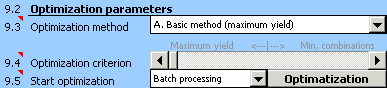
4) Press the button on line [9.5] to start optimization.
5) Basic qualitative parameters of the design procedure are specified in paragraph [9.6]
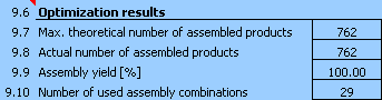
a detailed specification of optimized assembly procedure is shown in table [9.12].
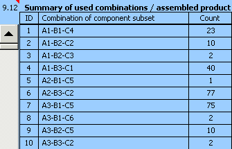
The left column of the table shows all assembly combinations used for assembly of the product. The right column shows the number of products assembled within each combination.
|
Optimization method |
Number of assembled bearings |
Number of used assembly combinations |
Speed of calculation |
|
A. Basic method |
762 |
29 |
6 min 20 s |
|
B. Modified method |
760 |
34 |
1 min 30 s |
|
C. Simplified method |
759 |
32 |
55 s |
Information on setting of calculation parameters and setting of the language can be found in the document "Setting calculations, change the language".
General information on how to modify and extend calculation workbooks is mentioned in the document "Workbook (calculation) modifications".
^